Acknowledgement: I am deeply grateful to my friends and colleagues who helped review this manuscript, namely Thijs van der Plas, Jiahao Zhang, Wenbo Jing, and Yingjie Shao.

Generative diffusion models reframe sample generation as an iterative denoising process: starting from pure Gaussian noise, they learn to reverse a carefully designed forward diffusion that gradually corrupts data.

This blog presents a unified derivation of two foundational approaches---Denoising Diffusion Probabilistic Models (DDPM) and Denoising Diffusion Implicit Models (DDIM)---tracing them from their variational autoencoder roots. We show how the training objective emerges naturally from the evidence lower bound (ELBO), reducing to a simple noise-prediction loss, and how the sampling procedure can be understood through its connection to score matching. Within this unified view, DDIM arises as a deterministic limit of DDPM, enabling accelerated sampling through a non-Markovian forward process while preserving the same marginal distributions and training objective.

Prefix

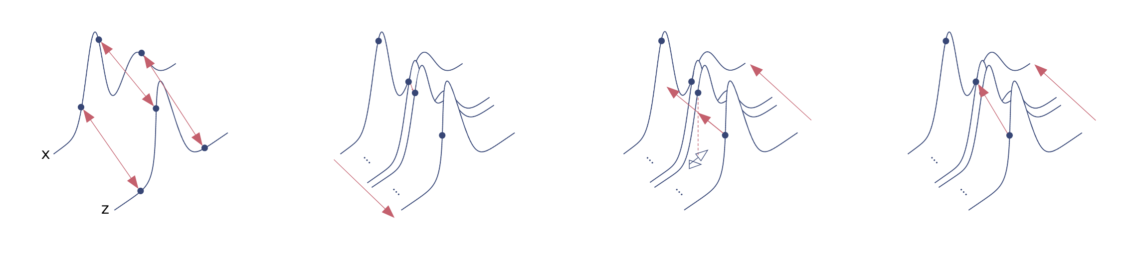
Generative models can be viewed as the processes that sample from an unknown data distribution. In image generation, the data distribution represents all possible images, while in language generation it is the distribution over possible sequences of text. In this blog, we adopt this perspective to re-derive the formalism of a class of image generation models—specifically diffusion models, including denoising diffusion probabilistic models (DDPM) and denoising diffusion implicit models (DDIM)—which form the basis of state-of-the-art systems such as Stable Diffusion and DALL·E.

Intuitively, one might consider a Monte Carlo approach in which samples are drawn from a simple, known distribution and only those consistent with the target data distribution are retained. However, such naive rejection sampling from a simple proposal distribution is infeasible in high dimensions, as the probability of accepting a sample becomes vanishingly small. Suppose we want to generate an RGB image of size $(512, 512)$ ; the dimensionality of the space is $512 \times 512 \times 3$ , and each dimension takes values in $\{0, 1, ..., 255\}$ . Since natural images lie on a highly structured, low-dimensional subset of this space, most samples from a simple distribution are very unlikely to correspond to realistic images, making such approaches extremely inefficient.

A more efficient approach is to learn a transformation from a known, easy-to-sample distribution to the target distribution, so that each sample corresponds to a generated data point. Many approaches have been proposed to learn such transformations. For example, in Generative Adversarial Networks (GANs), a generator is trained adversarially against a discriminator to produce samples that match the target distribution, effectively discouraging samples that deviate from the data distribution. In Variational Autoencoders (VAEs), an encoder–decoder architecture is defined within a Bayesian framework, and the model is trained by maximizing a lower bound on the data likelihood. In DDPM, we explicitly define a forward Markov process that gradually transforms data into Gaussian noise, and learn the reverse process to generate data from noise. Training can be interpreted as maximizing a variational lower bound on the data likelihood, similar in the spirit of VAEs.

The following sections introduce diffusion models and their related methods. We first review the ELBO derivation through VAEs (Section VAE), then derive DDPM (Section DDPM) and DDIM (Section DDIM). Finally, we discuss connections to score-based models (Section Score).

When writing this essay, I also read and learned a lot from several blog posts, including:

Notations

For convenience of later derivations, we list the required notations below.

Data and distributions

$x$ , $x_0$ : data point drawn from the target distribution
$p_{\text{data}}(x)$ : unknown target distribution we want to sample from
$p_\theta(x)$ : learned model distribution parameterized by $\theta$
$z$ : latent variable drawn from a simple prior
$p(z)$ : prior distribution, usually $\mathcal{N}(0, I)$
$p(x, z)$ : joint distribution of $x$ and $z$
$p(x \mid z)$ : conditional distribution of data given latent variable

Variational Inference (VAE)

$\phi, \theta$ : encoder and decoder parameters
$q_\phi(z \mid x)$ : approximate posterior (encoder)
$p_\theta(x \mid z)$ : decoder / likelihood
$\mu_\phi(x), \sigma_\phi^2(x)$ : encoder outputs

Distributions and metrics

$\mathcal{N}(\mu, \Sigma)$ : Gaussian distribution
$D_{KL}(P \parallel Q)$ : KL divergence
$\mathbb{E}_q[\cdot]$ : expectation under $q$

DDPM & diffusion process

$t$ : timestep in $\{1, \dots, T\}$
$x_t$ : latent variable at timestep $t$
$\alpha_t$ : noise schedule coefficient
$\bar{\alpha}_t = \prod_{s=1}^t \alpha_s$
$\epsilon_t \sim \mathcal{N}(0, I)$ : Gaussian noise
$q(x_t \mid x_{t-1})$ : forward process
$p_\theta(x_{t-1} \mid x_t)$ : learned reverse process
$\hat{\epsilon}_\theta(x_t, t)$ : noise prediction network
$\mu_\theta(x_t, t)$ : predicted reverse mean

DDIM

$\sigma_t$ : stochasticity parameter
$S$ : number of sampling steps
$\tau$ : subset of timesteps
$q_\sigma$ : DDIM sampling distribution

Score-based models

$\nabla_x \log p(x)$ : score function
$s_\theta(x, t)$ : learned score network
$\eta_t$ : noise scale
$p_t(x_t)$ : noisy marginal distribution
$\lambda(t)$ : weighting function

Langevin dynamics

$\gamma$ : step size
$z_t \sim \mathcal{N}(0, I)$ : injected noise
$n$ : timestep index for score updates

Variational AutoEncoders

In this section, we discuss the foundations of diffusion models, along with key aspects of their implementation, including the learning objective and how it is derived. Due to page limitations, some topics—such as text guidance—are not covered.

As discussed earlier, one common approach to generative modeling is to learn a transformation from a known, easy-to-sample distribution $p(z)$ to an unknown data distribution $p_{\text{data}}(x)$ , which describes real data.

In general, this transformation is not available in closed form. Instead, it can be learned by defining a trainable objective (i.e., a loss function) that measures the difference between the model distribution $p_{\theta}(x)$ and the data distribution $p_{\text{data}}(x)$ , and optimizing it using a neural network. The optimal parameters then define a model that approximates the target distribution. Ifgn this way, the problem of generating data is reduced to defining and solving an optimization problem.

Assumption 1
There exists a sufficiently regular transformation from $p(z)$ to $p_{\text{data}}(x)$ that can be approximated by a neural network.

Assumption 1 ensures that the model has enough expressive power to represent the target distribution. This assumption is nontrivial, since not every pair of distributions can be related through such a transformation in a well-behaved manner. For example, when the target distribution is singular (such as a Dirac delta distribution) while the model distribution is continuous (such as a Gaussian), the Kullback--Leibler divergence can become infinite, indicating a fundamental mismatch between the two distributions. In such cases, directly approximating the target distribution can be challenging.

We now turn to how to define the optimization problem. For simplicity, we use a Gaussian distribution as the base distribution $p(z)$ , leveraging its convenient mathematical properties.

Evidence Lower Bound (ELBO)

To define the optimization problem, a natural approach is to use likelihood-based learning. Given a dataset $\{x_i\}_{i=1}^N$ , the objective is to maximize the likelihood of the data under the model, i.e., maximize $p_\theta(x_i)$ for all samples. A naive approach might be to sample latent variables $z_i$ from a Gaussian distribution and arbitrarily associate them with data samples $x_i$ , then optimize the likelihood based on these random pairings. However, this approach is flawed because such random pairings do not establish a meaningful relationship between the latent variables and the data samples. As a result, the model cannot learn how changes in the latent space correspond to variations in the data. Instead, it may rely on overall statistics of the dataset and largely ignore the latent variables. Under common training objectives, this can lead to outputs that resemble an average of the data distribution, rather than distinct and realistic samples.

This issue suggests that, to learn a meaningful transformation, it is not sufficient to consider only the marginal likelihood $p_\theta(x)$ . Instead, we should explicitly model the relationship between $x$ and $z$ . To achieve this, we introduce the conditional distribution $p(x \mid z)$ , which describes how a data point $x$ is generated from a latent variable $z$ . This provides the necessary structure to guide the learning process and establish a meaningful mapping between the latent space and the data space.

We introduce a variational distribution $q_\phi(z \mid x)$ to approximate the intractable posterior $p(z \mid x)$ , where $\phi$ denotes the parameters to be optimized. This allows us to reformulate the objective in terms of the marginal likelihood $p_\theta(x)$ and work with its logarithm, $\log p_\theta(x)$ , which is more convenient for optimization.

Consider log likelihood:

\begin{align} \log p(x) &= \log p(x) \int q_{\phi}(z \mid x)\, dz \\ &= \int \log p(x)\, q_{\phi}(z \mid x)\, dz \\ &= \mathbb{E}_{q_{\phi}(z \mid x)} \left[ \log p(x) \right] \\ &= \mathbb{E}_{q_{\phi}(z \mid x)} \left[ \log \frac{p(x, z)}{p(z \mid x)} \right] \\ &= \mathbb{E}_{q_{\phi}(z \mid x)} \left[ \log \frac{p(x, z)}{p(z \mid x)} \cdot \frac{q_{\phi}(z \mid x)}{q_{\phi}(z \mid x)} \right] \\ &= \mathbb{E}_{q_{\phi}(z \mid x)} \left[ \log \frac{p(x, z)}{q_{\phi}(z \mid x)} + \log \frac{q_{\phi}(z \mid x)}{p(z \mid x)} \right] \\ &= \mathbb{E}_{q_{\phi}(z \mid x)} \left[\log \frac{p(x, z)}{q_{\phi}(z \mid x)}\right] + D_{KL} (q_{\phi}(z \mid x) \lVert p(z \mid x)) \\ &\geq \mathbb{E}_{q_{\phi}(z \mid x)} \left[\log \frac{p(x, z)}{q_{\phi}(z \mid x)}\right] \end{align} \tag{1}

The derivation shows that it can be expressed as the sum of a lower bound and a KL divergence term between the approximate posterior and the true posterior. Since the KL divergence is non-negative, the resulting expression provides a lower bound on $\log p_\theta(x)$ , which is referred to as the Evidence Lower Bound (ELBO). The ELBO is used as the optimization objective in VAEs. This is motivated by two key reasons. First, it provides a tractable lower bound on the log-likelihood, and maximizing it indirectly improves the data likelihood. Second, it introduces a framework for learning a structured latent representation, where we explicitly model how data points are generated from latent variables. Although the exact KL term between the approximate posterior and the true posterior is intractable, maximizing the ELBO avoids computing it directly. Since $\log p_\theta(x)$ does not depend on $\phi$ , maximizing the ELBO is equivalent to making the approximate posterior closer to the true posterior.

We now rewrite the ELBO in a more interpretable form.

\begin{align} \mathbb{E}_{q_{\phi}(z \mid x)} \left[\log \frac{p(x, z)}{q_{\phi}(z \mid x)}\right] &= \mathbb{E}_{q_{\phi}(z \mid x)} \left[\log \frac{p(x|z)p(z)}{q_{\phi}(z \mid x)}\right] \\ &= \mathbb{E}_{q_{\phi}(z \mid x)} \log p(x|z) + \mathbb{E}_{q_{\phi}(z \mid x)} \left[\log\left(\frac{p(z)}{q_{\phi}(z \mid x)}\right)\right] \\ &= \mathbb{E}_{q_{\phi}(z \mid x)} \left[\log p(x|z)\right] - D_{KL} (q_{\phi}(z \mid x) \lVert p(z)) \end{align} \tag{2}

The resulting expression consists of two terms. The first term corresponds to a reconstruction objective, which encourages accurate generation of data from latent variables. The second term is a KL divergence between the approximate posterior $q_\phi(z \mid x)$ and the prior $p(z)$ , which regularizes the latent representation to stay close to a simple distribution.

In practice, this objective is optimized using two neural networks: one parameterizing the encoder $q_\phi(z \mid x)$ , and the other parameterizing the decoder $p_\theta(x \mid z)$ .

Training and Reparameterization

We just introduced ELBO, following we explain how a VAE is trained to maximize it. In VAEs, the encoder is modeled as a Gaussian distribution parameterized by $\phi$ , while the prior distribution over the latent variable is chosen to be a standard Gaussian:

\begin{align} q_{\phi}(z \mid x) = \mathcal{N}(\mu_{\phi}(x), \sigma_{\phi}^{2}(x)); \\ \qquad \\ p(z) = \mathcal{N}(0, I) \end{align} \tag{3}

Therefore, the encoder is trained to predict the mean and variance of the latent variable $z$ given a data sample $x$ .

The reconstruction term in the ELBO can be approximated using Monte Carlo sampling with latent variables sampled from $q_{\phi}(z \mid x)$ . However, the sampling operation itself is not differentiable, preventing gradients from being propagated through the network during backpropagation. To address this issue, we use the reparameterization trick. Instead of directly sampling from $\mathcal{N}(\mu_{\phi}(x), \sigma_{\phi}^{2}(x))$ , we first sample

\epsilon \sim \mathcal{N}(0, I), \tag{4}

and then compute

\begin{align} z = \mu_{\phi}(x) + \sigma_{\phi}(x) \odot \epsilon \end{align} \tag{5}

where $\odot$ denotes element-wise multiplication.

After training, the VAE consists of an encoder $q_\phi(z \mid x)$ and a decoder $p_\theta(x \mid z)$ . To generate new data, we first sample a latent variable $z$ from the prior distribution $\mathcal{N}(0, I)$ and then pass it through the decoder $p_\theta(x \mid z)$ . In the generation process, only the decoder is used to produce samples, while the encoder is introduced during training to establish the relationship between the data space and the latent space.

Denoising Diffusion Probabilistic Models (DDPM)

Previously, we saw that in variational autoencoders (VAEs), the transformation from a known prior distribution to the data distribution is learned implicitly through an encoder–decoder pair. A limitation of this approach is that the relationship between data and latent variables is only captured through an approximate posterior, which introduces additional modeling and inference complexity.

An alternative approach is to construct a stepwise transformation from the data distribution to a Gaussian distribution. Intuitively, this can be understood as forming a linear combination of the original data and Gaussian noise. Over time, the contribution of the noise gradually increases while the contribution of the data decreases, eventually resulting in pure Gaussian noise.

Equivalently, this process can be defined as a stepwise Markov chain. For convenience, we introduce the following notation:

$x_0$ : original data sample
$x_T$ : latent variable at the final timestep (standard Gaussian noise)
$x_t$ : intermediate latent state at timestep $t$

where $t \in {0, \dots, T}$ .

Under this notation, the forward process is defined as

x_t = \sqrt{\alpha_t} , x_{t-1} + \sqrt{1 - \alpha_t},\epsilon_t, \qquad \epsilon_t \sim \mathcal{N}(0,I). \tag{6}

By recursively applying this relation, we can express $x_t$ in terms of the original data $x_0$ . For example,

\begin{aligned} x_t &= \sqrt{\alpha_t} \left( \sqrt{\alpha_{t-1}}x_{t-2} + \sqrt{1-\alpha_{t-1}}\epsilon_{t-1} \right) + \sqrt{1-\alpha_t}\epsilon_t \\ &= \sqrt{\alpha_t\alpha_{t-1}},x_{t-2} + \sqrt{\alpha_t(1-\alpha_{t-1})},\epsilon_{t-1} + \sqrt{1-\alpha_t},\epsilon_t. \end{aligned} \tag{7}

Continuing this expansion yields a weighted sum of independent Gaussian noises. Since a linear combination of independent Gaussian random variables is still Gaussian, we can merge the noise terms into a single Gaussian random variable $\epsilon \sim \mathcal{N}(0,I)$ .

The merged variance is

\sigma^2 = \alpha_t(1-\alpha_{t-1}) + (1-\alpha_t) = 1-\alpha_t\alpha_{t-1}. \tag{8}

Repeating this process until $t=0$ yields the closed-form expression

x_t = \sqrt{\bar{\alpha}_t},x_0 + \sqrt{1-\bar{\alpha}_t},\epsilon, \tag{9}

where

\bar{\alpha}_t = \prod_{s=1}^{t}\alpha_s, \qquad \epsilon \sim \mathcal{N}(0,I). \tag{10}

This formulation shows that the forward process gradually destroys the structure of the data, and after sufficiently many steps, the distribution of $x_T$ approaches a standard Gaussian distribution.

Formulation of the Diffusion Process

We now summarize the diffusion process more formally.

To make the stepwise noising process meaningful, we assume that the transformation from the data distribution to a Gaussian distribution can be approximated through a sequence of small stochastic transitions. This assumption differs from Assumption 1, since the forward diffusion process is explicitly defined rather than learned by a neural network.

Several important assumptions and design choices are made in this formulation:

Markov Property
The forward process is assumed to satisfy the Markov property, meaning each state depends only on the previous state. This allows the joint distribution of the trajectory to be written as
$q(\mathbf{x}\mid x_0) = \prod_{t=1}^{T} q(x_t\mid x_{t-1}). \tag{11}$
Gaussian Transitions
Each transition is modeled as a Gaussian distribution, which enables the forward process to admit the closed-form expression derived above.
Variance-Preserving Process
The coefficients are chosen such that the overall scale of the samples remains stable throughout the diffusion process, preventing the signal from growing or shrinking uncontrollably.
Gaussian Terminal Distribution
After sufficiently many diffusion steps, the final state $x_T$ approaches a standard Gaussian distribution.

If we could reverse this process and iteratively sample from the reverse conditional distribution $q(x_{t-1}\mid x_t)$ , we would be able to generate samples from the data distribution starting from Gaussian noise.

However, this reverse conditional is generally intractable to compute directly. Therefore, diffusion models instead learn a parameterized model $p_\theta(x_{t-1}\mid x_t)$ to approximate the reverse diffusion process.

ELBO in Diffusion Models

We now have all the necessary components to formulate the diffusion model objective.

Unlike VAEs, the forward process $q(x_t \mid x_{t-1})$ is no longer parameterized by $\phi$ , but is instead explicitly defined as a fixed stochastic process. As a result, the learning problem focuses only on the reverse process $p_\theta(x_{t-1}\mid x_t)$ , which serves as the generative component of the model.

Similar to the VAE formulation, we can derive a variational lower bound (ELBO) for the log-likelihood objective. The detailed derivation and intermediate steps are provided in the appendix.

\log p(x_0) \ge \mathbb{E}_{q(\mathbf{x}\mid x_0)} \left[ \log \frac{ p(x_{0:T}) }{ q(\mathbf{x}\mid x_0) } \right] = \mathbb{E}_{q(\mathbf{x}\mid x_0)} \left[ \log \frac{ p(x_T)\prod_{t=1}^{T}p_\theta(x_{t-1}\mid x_t) }{ \prod_{t=1}^{T}q(x_t\mid x_{t-1}) } \right]. \tag{12}

After a sequence of algebraic manipulations, the ELBO can be written as

\begin{aligned} & \mathbb{E}_{q(x_1\mid x_0)} \log p_\theta(x_0\mid x_1) \\ &- D_{KL} \left( q(x_T\mid x_0) \parallel p(x_T) \right) \\ &- \sum_{t=2}^{T} \mathbb{E}_{q(x_t\mid x_0)} D_{KL} \left( q(x_{t-1}\mid x_t,x_0) \parallel p_\theta(x_{t-1}\mid x_t) \right). \end{aligned} \tag{13}

The terms in the above expression can be interpreted as follows:

Reconstruction term
$\mathbb{E}_{q(x_1\mid x_0)} \log p_\theta(x_0\mid x_1) \tag{14}$
measures how well the model can recover the original data from a slightly noisy sample, analogous to the reconstruction objective in VAEs.
Prior matching term
$D_{KL} \left( q(x_T\mid x_0) \parallel p(x_T) \right) \tag{15}$
measures how close the final distribution of the forward diffusion process is to a standard Gaussian distribution. By construction, and for sufficiently large $T$ , this term is effectively constant during training.
Denoising matching term
$\mathbb{E}_{q(x_t\mid x_0)} D_{KL} \left( q(x_{t-1}\mid x_t,x_0) \parallel p_\theta(x_{t-1}\mid x_t) \right) \tag{16}$
trains the reverse process to approximate the true reverse posterior.

The reverse posterior is Gaussian and can be written as

q(x_{t-1}\mid x_t,x_0) = \mathcal{N} \left( x_{t-1}; \mu_q(x_t,x_0), \Sigma_q(t) \right), \tag{17}

where

\mu_q(x_t,x_0) = \frac{ \sqrt{\alpha_t}(1-\bar{\alpha}_{t-1})x_t + \sqrt{\bar{\alpha}_{t-1}}(1-\alpha_t)x_0 }{ 1-\bar{\alpha}_t }. \tag{18}

and

\Sigma_q(t) = \frac{ (1-\alpha_t)(1-\bar{\alpha}_{t-1}) }{ 1-\bar{\alpha}_t }. \tag{19}

Training the Diffusion Model and Sampling

Recall that the KL divergence between two Gaussian distributions simplifies considerably when their covariance matrices are fixed to be equal.

In that case, minimizing

D_{KL} \left( q(x_{t-1}\mid x_t,x_0) \parallel p_\theta(x_{t-1}\mid x_t) \right) \tag{20}

is equivalent to minimizing the squared error between their means:

\arg\min_\theta \left\| \mu_\theta(x_t,t) - \mu_q(x_t,x_0) \right\|_2^2. \tag{21}

Using the forward-process relation

x_t = \sqrt{\bar{\alpha}_t}x_0 + \sqrt{1-\bar{\alpha}_t}\epsilon, \tag{22}

we can solve for $x_0$ :

x_0 = \frac{ x_t - \sqrt{1-\bar{\alpha}_t},\epsilon }{ \sqrt{\bar{\alpha}_t} }. \tag{23}

Substituting this into the posterior mean yields

\mu_q(x_t,x_0) = \frac{1}{\sqrt{\alpha_t}} \left( x_t - \frac{1-\alpha_t}{\sqrt{1-\bar{\alpha}_t}} \epsilon \right). \tag{24}

This suggests that, instead of directly predicting the posterior mean, we can train a neural network $\hat{\epsilon}_\theta(x_t,t)$ to predict the noise added at timestep $t$ .

The resulting optimization objective becomes

\arg\min_\theta \mathbb{E}_{x_0,\epsilon,t} \left[ \lambda(t) \left\| \epsilon - \hat{\epsilon}_\theta \left( \sqrt{\bar{\alpha}_t}x_0 + \sqrt{1-\bar{\alpha}_t}\epsilon, t \right) \right\|_2^2 \right]. \tag{25}

Here $\lambda(t)$ denotes the weighting term induced by the KL divergence.

In the simplified DDPM objective, $\lambda(t)$ is commonly set to $1$ , which empirically leads to improved sample quality.

In practice, the reconstruction term is also absorbed into the simplified denoising objective. Consequently, training is dominated by the noise-prediction loss, which teaches the model to estimate the Gaussian noise added at each diffusion timestep.

Training and Sampling Algorithm

In reverse sampling, $\sigma_t$ is a tunable hyperparameter that controls how much random noise is injected at each timestep.

The overall training procedure of diffusion models can now be summarized as follows.

During training, we first sample a real data point $x_0$ from the dataset and randomly choose a timestep $t \in {1,\dots,T}$ . Gaussian noise is then added according to

x_t = \sqrt{\bar{\alpha}_t}x_0 + \sqrt{1-\bar{\alpha}_t}\epsilon. \tag{26}

The noisy sample $x_t$ , together with the timestep $t$ , is passed into the neural network $\hat{\epsilon}_\theta(x_t,t)$ , which is trained to predict the noise $\epsilon$ that was added to the original data.

Because the timestep is sampled uniformly during training, the model learns to denoise samples across a wide range of noise levels.

After training, generation proceeds through the reverse diffusion process. We first sample $x_T \sim \mathcal{N}(0,I)$ , which corresponds to pure Gaussian noise.

The learned model then iteratively predicts and removes noise from the sample:

x_T \rightarrow x_{T-1} \rightarrow \cdots \rightarrow x_1 \rightarrow x_0. \tag{27}

At each timestep, the model predicts the noise component in the current sample and uses it to estimate a less noisy sample from the previous timestep. After sufficiently many reverse steps, the final sample $x_0$ approximately follows the data distribution, producing a generated image.

Denoising Diffusion Implicit Models (DDIM)

The derivation of diffusion models follows a progressive sequence of steps:

q(\mathbf{x}_t \mid \mathbf{x}_{t-1}) \xrightarrow{\text{Derivation}} q(\mathbf{x}_t \mid \mathbf{x}_0) \xrightarrow{\text{Deration}} q(\mathbf{x}_{t-1} \mid \mathbf{x}_t, \mathbf{x}_0) \xrightarrow{\text{Approximation}} p_\theta(\mathbf{x}_{t-1} \mid \mathbf{x}_t). \tag{28}

Although the derivation is constructed through a stepwise Markov process, the final formulation exhibits two important characteristics:

Loss Function Independence:
The training objective depends only on the marginal distribution $q(\mathbf{x}_t \mid \mathbf{x}_0)$ .
Sampling Independence:
The sampling procedure depends only on the learned reverse process $p_\theta(\mathbf{x}_{t-1} \mid \mathbf{x}_t)$ .

This observation suggests that the explicit Markovian structure of the forward process is not essential for defining the training objective. As long as the marginal distributions $q(\mathbf{x}_t \mid \mathbf{x}_0)$ remain unchanged, different forward processes can lead to the same optimization objective. DDIM extends this idea by introducing a more general non-Markovian diffusion process.

DDIM Sampling and Non-Markovian Diffusion

In DDPM, the marginal distribution of $x_t$ conditioned on $x_0$ is Gaussian:

q(x_t \mid x_0) = \mathcal{N} \left( x_t; \sqrt{\bar{\alpha}_t}x_0, (1-\bar{\alpha}_t)I \right) \tag{29}

DDIM considers a non-Markovian forward process while preserving the same marginal distribution $q(x_t \mid x_0)$ . The goal remains to generate $x_0$ starting from Gaussian noise $x_T$ . Unlike DDPM, where each reverse step involves sampling from a probability distribution, DDIM introduces an implicit deterministic mapping

x_{t-1} = f(x_t, t). \tag{30}

From Eq. (29), we have the expression for $x_0$ . After training a DDPM model, a neural network can be used to approximate the noise component $\epsilon_t$ with $\hat{\epsilon}_\theta(x_t,t)$ . Therefore, both the original and estimated forms of $x_0$ can be written as

x_0 = \frac{1}{\sqrt{\bar{\alpha}_t}} \left( x_t - \sqrt{1-\bar{\alpha}_t}\,\epsilon_t \right), \qquad \hat{x}_0 = \frac{1}{\sqrt{\bar{\alpha}_t}} \left( x_t - \sqrt{1-\bar{\alpha}_t}\, \hat{\epsilon}_\theta(x_t,t) \right) \tag{31}

Applying the diffusion relation again at timestep $t-1$ gives

x_{t-1} = \sqrt{\bar{\alpha}_{t-1}}x_0 + \sqrt{1-\bar{\alpha}_{t-1}}\epsilon_{t-1}. \tag{32}

DDIM further decomposes the noise term into a deterministic component and a stochastic component:

x_{t-1} = \sqrt{\bar{\alpha}_{t-1}}x_0 + \sqrt{1-\bar{\alpha}_{t-1}-\sigma_t^2} \,\hat{\epsilon}_\theta(x_t,t) + \sigma_t\epsilon, \tag{33}

where $\epsilon \sim \mathcal{N}(0,I)$ .

Substituting Eq. (31) into Eq. (33) gives

x_{t-1} = \sqrt{\bar{\alpha}_{t-1}} \left( \frac{ x_t - \sqrt{1-\bar{\alpha}_t}\, \hat{\epsilon}_\theta(x_t,t) }{ \sqrt{\bar{\alpha}_t} } \right) + \sqrt{1-\bar{\alpha}_{t-1}- \sigma_t^2} \,\hat{\epsilon}_\theta(x_t,t) + \sigma_t\epsilon. \tag{34}

Eq. (34) defines the DDIM sampling process:

q_\sigma(x_{t-1} \mid x_t, x_0) = \mathcal{N} \Bigl( x_{t-1}; \mu_\sigma(x_t,x_0), \sigma_t^2 I \Bigr) \tag{35}

where the mean term in Eq. (35) is

\mu_\sigma(x_t,x_0) = \sqrt{\bar{\alpha}_{t-1}} \left( \frac{ x_t - \sqrt{1-\bar{\alpha}_t}\, \hat{\epsilon}_\theta(x_t,t) }{ \sqrt{\bar{\alpha}_t} } \right) + \sqrt{1-\bar{\alpha}_{t-1}-\sigma_t^2} \,\hat{\epsilon}_\theta(x_t,t). \tag{36}

We can treat $\sigma_t^2$ as a hyperparameter that controls the stochasticity of the sampling process in Eq. (35). When $\sigma_t^2 = 0$ , the sampling process becomes fully deterministic. When

\sigma_t^2 = \frac{1-\bar{\alpha}_{t-1}}{1-\bar{\alpha}_t} (1-\alpha_t), \tag{37}

the sampling process in Eq. (35) reduces to the original DDPM formulation.

During generation, it is not necessary to follow the entire sequence of timesteps $\{1,\dots,T\}$ . Instead, we may sample using only a subset of timesteps. Let $m < n$ denote two timesteps in this trajectory. The DDIM reverse update step is then given by Eq. (38),

\begin{aligned} & q_{\sigma, m < n} (\mathbf{x}_m \mid \mathbf{x}_n, \mathbf{x}_0)\\ & = \mathcal{N} \Bigg( \mathbf{x}_m; \sqrt{\bar{\alpha}_m} \left( \frac{ \mathbf{x}_n - \sqrt{1-\bar{\alpha}_n} \hat{\epsilon}_\theta^{(n)}(\mathbf{x}_n, n) }{ \sqrt{\bar{\alpha}_n} } \right) + \sqrt{1-\bar{\alpha}_m-\sigma_n^2} \, \hat{\epsilon}_\theta^{(n)}(\mathbf{x}_n, n), \, \sigma_n^2 \mathbf{I} \Bigg) \tag{38} \end{aligned}

This formulation gives DDIM two important advantages over DDPM:

By controlling the parameter $\sigma_t$ , the sampling process can interpolate between stochastic and deterministic generation.
Since sampling does not need to follow the full sequence of timesteps, generation can be performed using only a subset (Eq. (39))

\tau = \{\tau_1,\dots,\tau_S\}, \qquad S \ll T, \tag{39}

which significantly reduces the computational cost while maintaining comparable sample quality.

Connection to Score-based Models

Having introduced the basics of diffusion models, we now show the connection between diffusion models and score-based generative models.

Directly modeling the likelihood function $p(x)$ is often intractable, and estimating it using methods such as Markov chain Monte Carlo (MCMC) or variational inference can be computationally expensive. Score-based models address this difficulty by modeling the score function instead of the probability density itself. The score function of a distribution is defined as

\nabla_x \log p(x). \tag{40}

Rather than learning the density function directly, score-based models learn the gradient of the log-density. Similar to other likelihood-based generative models, such as VAEs, the objective is still related to maximizing likelihood, but the optimization is performed through score matching. The corresponding objective minimizes the Fisher divergence:

\mathbb{E}_{p(x)} \left[ \left\| \nabla_x \log p(x) - s_\theta(x) \right\|_2^2 \right], \tag{41}

where $s_\theta(x)$ denotes the learned score function.

An important advantage of score-based models is that they do not require a tractable normalizing constant for the probability density. Instead, the model directly learns a vector field describing the direction of increasing probability density.

However, score estimation in low-density regions is often inaccurate. Expanding the Fisher divergence gives

\mathbb{E}_{p(x)} \left[ \left\| \nabla_x \log p(x) - s_\theta(x) \right\|_2^2 \right] = \int p(x) \left\| \nabla_x \log p(x) - s_\theta(x) \right\|_2^2 \, dx \tag{42}

Since the weighting term $p(x)$ is small in low-density regions, errors in these regions contribute little to the optimization objective. As a result, the learned score function is often inaccurate far from the data manifold.

Score-based Modeling with Multiple Noise Perturbations

To address this issue, score-based models perturb the data with Gaussian noise and train the score function on the perturbed distributions instead. Large noise levels improve coverage of low-density regions, while small noise levels preserve the structure of the original data distribution.

To balance these effects, multiple noise scales are introduced. Let $\{\eta_t\}_{t=1}^{T}$ denote a sequence of noise levels. Given a data sample $x \sim p(x)$ , we generate a perturbed sample

x_t = x + \eta_t \epsilon, \qquad \epsilon \sim \mathcal{N}(0,I) \tag{43}

The resulting perturbed distribution is

p_t(x_t) = \int p(y)\, \mathcal{N}(x_t; y, \eta_t^2 I)\, dy \tag{44}

A noise-conditional score network (NCSN) is then trained to estimate the score function at different noise levels. The training objective becomes

\sum_{t=1}^{T} \lambda(t) \mathbb{E}_{p_t(x_t)} \left[ \left\| \nabla_{x_t}\log p_t(x_t) - s_\theta(x_t,t) \right\|_2^2 \right]. \tag{45}

Equivalence to Diffusion Models

The connection between score-based models and diffusion models comes from the fact that predicting the noise added to a sample is equivalent to estimating the score function.

In diffusion models, the forward conditional from Eq. (29) is $p(x_t \mid x_0)=\mathcal{N}\bigl(x_t;\, \sqrt{\bar{\alpha}_t}x_0,\, (1-\bar{\alpha}_t)I\bigr)$ . Differentiating the log-density with respect to $x_t$ yields

\nabla_{x_t}\log p(x_t \mid x_0) = -\frac{x_t - \sqrt{\bar{\alpha}_t}x_0}{1-\bar{\alpha}_t}. \tag{46}

With the usual reparameterization from Eq. (22), $x_t = \sqrt{\bar{\alpha}_t}x_0 + \sqrt{1-\bar{\alpha}_t}\,\epsilon$ , this becomes

\nabla_{x_t}\log p(x_t \mid x_0) = -\frac{\epsilon}{\sqrt{1-\bar{\alpha}_t}}. \tag{47}

Substituting into the score-matching objective and comparing with the DDPM noise-prediction loss in Eq. (25), we consider

\sum_{t=1}^{T}\lambda(t)\, \mathbb{E}\left[ \left\| -\frac{\epsilon}{\sqrt{1-\bar{\alpha}_t}} - s_\theta(x_t,t) \right\|_2^2 \right] \quad\text{and}\quad \mathbb{E}_{t,x_0,\epsilon} \left[ \left\| \epsilon - \hat{\epsilon}_\theta(x_t,t) \right\|_2^2 \right]. \tag{48}

These differ only by a scaling factor; in particular,

s_\theta(x_t,t) \approx -\frac{\hat{\epsilon}_\theta(x_t,t)}{\sqrt{1-\bar{\alpha}_t}}. \tag{49}

Therefore, training a diffusion model to predict noise is equivalent to training a score-based model.

Once the score is learned, one may sample using Langevin dynamics, where $t$ denotes the outer iterate index:

x_{t+1} = x_t + \gamma \nabla_x \log p(x_t) + \sqrt{2\gamma}\, z_t, \qquad z_t \sim \mathcal{N}(0,I). \tag{50}

Replacing $\nabla_x \log p$ by the diffusion noise predictor at diffusion timestep $n$ gives

x_{t+1} \approx x_t - \gamma \, \frac{\hat{\epsilon}_\theta(x_t,n)}{\sqrt{1-\bar{\alpha}_n}} + \sqrt{2\gamma}\, z_t. \tag{51}

This highlights the close relationship between score-based sampling and diffusion-model denoising.

In the continuous-time limit, diffusion can be written as a stochastic differential equation (SDE), and the reverse process (together with a deterministic probability-flow ODE) links DDPM- and DDIM-style sampling to score-based dynamics.